Processing Your Data
Why It Matters
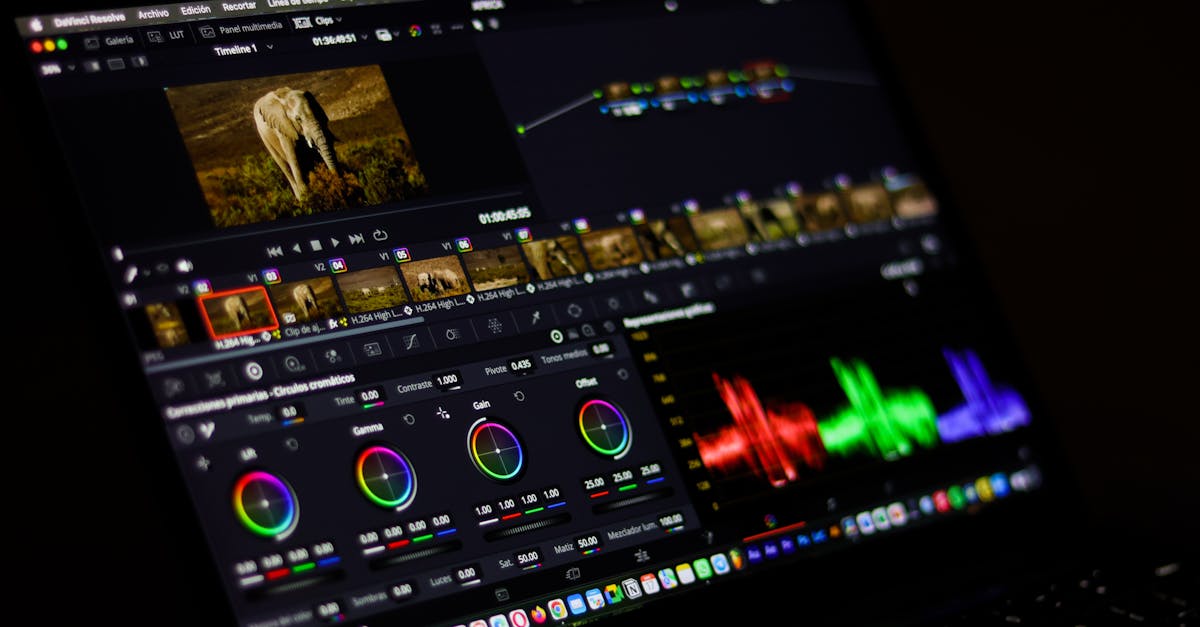
You’ve flown the mission, captured 500 carefully planned photos, and downloaded everything. Now the real work begins. Processing converts your raw data into usable outputs. Understanding the pipeline determines whether your results are accurate or just pretty pictures.
Each step in the pipeline affects final accuracy. Understanding these steps helps you diagnose problems and optimize results.
The Processing Pipeline
Step 1: Import and Inspect
Import your photos into the processing software. Before starting:
- Check image count: make sure all flights are included
- Remove bad photos: delete any that are blurry, severely over/underexposed, or show the drone’s landing gear
- Verify GPS data: confirm photos have geotags (latitude, longitude, altitude)
- Assign coordinate system: match the EPSG code used for your GCP survey
Step 2: Import GCP Data
Load your GCP coordinates and mark each GCP’s position in at least 3-5 photos. The software identifies the pixel location of each GCP center in multiple images and uses this to anchor the model.
This is a manual step. You click on the center of each GCP target in each photo where it’s visible. Accuracy here directly affects your final results.
Step 3: Image Alignment (Feature Matching)
The software analyzes every photo, identifies thousands of feature points (edges, corners, textures), and matches those features across overlapping images. Using these matches, it calculates the 3D position of each camera when each photo was taken.
Settings to check:
- Accuracy/Quality: “High” for production work, “Medium” for test runs
- Key point limit: 40,000-60,000 per image is typical
- Tie point limit: 4,000-6,000 per image
Output: a sparse point cloud and calibrated camera positions.
Time: 10-30 minutes for 500 photos on a good computer.
Step 4: Dense Point Cloud Generation
Based on the aligned cameras, the software generates a dense point cloud: millions of 3D points representing the terrain surface. This is the most computationally intensive step.
Settings to check:
- Quality: “High” for production (longer processing), “Medium” for drafts
- Depth filtering: “Mild” for complex geometry (buildings), “Aggressive” for flat terrain
- Point classification: enable if available, separates ground from buildings and vegetation
Output: millions of colored 3D points.
Time: 1-4 hours for 500 photos, depending on settings and hardware.
Step 5: Mesh Generation
The point cloud is connected into a 3D triangulated mesh, a surface made of millions of small triangles. The mesh provides the geometric framework for the orthomosaic and 3D model.
Settings:
- Face count: higher means more detail but larger files. 1-5 million faces is typical.
- Interpolation: “Enabled” fills small gaps; “Disabled” leaves holes where no data exists.
Step 6: Orthomosaic Generation
The original photos are projected onto the mesh surface and stitched into a single geometrically corrected image called the orthomosaic. Perspective distortion is removed, so the image is scale-accurate across the entire map.
Settings:
- Resolution: match your GSD or slightly lower
- Blending mode: “Mosaic” averages overlapping photos for even exposure; “Ortho” selects the most nadir photo per area
- Hole filling: enable for complete coverage
Output: a single large GeoTIFF file covering the entire mapping area.
Time: 30-60 minutes for most projects.
Step 7: DEM/DSM Generation
Elevation data is extracted from the point cloud:
- Digital Surface Model (DSM): all surface features (buildings, trees, vehicles)
- Digital Terrain Model (DTM): bare earth only (ground points after classification)
Output: GeoTIFF raster files where each pixel contains an elevation value.
Step 8: Export and Deliver
Export all outputs in appropriate formats:
- Orthomosaic: GeoTIFF, ECW, or JPEG with world file
- DEM/DSM: GeoTIFF
- Point cloud: LAS/LAZ format
- 3D model: OBJ, FBX, or KMZ (for Google Earth)
- Contours: DXF or Shapefile
Quick Check
Q: What is a dense point cloud? A: Millions of 3D points generated from aligned photos, representing the terrain surface with color and elevation data.
Q: Why is the GCP marking step done manually? A: Because accurately clicking the center of each GCP target in multiple photos is critical for absolute accuracy. The software can’t reliably auto-detect GCP centers with sufficient precision.
Q: What is the difference between DSM and DTM? A: DSM (Digital Surface Model) includes all surface features like buildings and trees. DTM (Digital Terrain Model) is bare earth only, with objects filtered out.
What’s Next?
Now let’s explore the specific outputs in detail (orthomosaics, DEMs, contour lines, 3D models) and how professionals use each one.